Copy and Paste Part 2: Formulas

This is the second in a series about copying and pasting in Excel.  It may seem a little too basic of a topic, but Excel offers several helpful pasting options that many folks do not even know exist. In this series, I will show y'all those features that I use regularly when working with my Evergreen reports.

In the previous post in this series, I talked about selecting multiple cells in Excel so you can copy and paste data throughout a table. The example I used in the video demonstration came from a question about step #5 in this handout where we must paste a formula in multiple cells.

What I did not happen to mention in the video was that Excel was doing more than just simple copying and pasting. It was not just taking the same data and duplicating it "verbatim" into each cell. Excel was taking the formula that I had copied and reconstructing it relative to each cell.

Now for simple numbers, text and dates, Excel handles copying and pasting like most other computer programs. It pastes the information exactly as it was copied, including any special formatting like font color, size, etc.  BUT for formulas, Excel does things differently. 



Take the following simple example:

For Excel to add the total, we type the following formula into B5:

  =SUM(B2:B4)

This will add up everything from B2 through B4,
giving us 15.



But there's a little more to know about the formula we just typed into B5:

It is using what is called relative cell references. We know this because we do not see the symbol "$" in the formula.  The "$" indicates absolute cell references, which we will talk about later.

Because the formula is using relative cell references, what the formula is really stating is "add together the 3 cells above me" ...as illustrated here.




We then add two more columns of data, which means we need the "add together the 3 cells above me" formula again:

All we need to do is simply copy B5, select the C5 and D5, and then paste!






Excel will automatically change the cell references relative to the cell in which you paste the formula:

(Toggle to view formulas, instead of values, by clicking Ctrl + `)

The automatic updating of cell references is a lovely feature of Excel.  It is so useful that relative cell references are the default for formula creation.  BUT sometimes you do not want Excel to change the cell reference when you are copying and pasting formulas.  This is when you want to use absolute cell references in a formula.

As I mentioned previously the "$" sign before a cell reference indicates that it is absolute. In other words, it is unchanging; it is not relative.  

• Both column and row references can be absolute ($A$1). 
• Or only the column reference, but the not the row ($A1). 
• Or vice versa (A$1).

Basically, whatever part of the reference you want to stay the same in the formula, regardless of where you move that formula, you must add a "$" before it. 

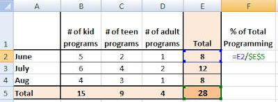
So to continue with this simple example, we have totaled the number of programs by month and by type, with the grand total in cell E5:

We now want to know how the programs were distributed across the months as a percentage of the total programs.  So we add a new header to column F and then add the following formula to cell F2:

=E2/$E$5

The first part of the formula uses relative cell reference and the second part uses absolute.  The formula translates to "divide the cell directly to my left by E5," as illustrated below:



Now when we copy and paste that formula into the cells below, Excel will change the cell references appropriately  in first part of the formula, but always use the grand total value in E5.

 









Now that we understand absolute and relative cell references, I can keep my promise and explain the formula I introduced in my last post: 
 

Copy and Paste Part 1: Selecting Multiple Cells

This is the first in a series about copying and pasting in Excel.  It may seem a little too basic of a topic, but Excel offers several helpful pasting options that many folks do not even know exist. In this series, I will show y'all those features that I use regularly when working with my Evergreen reports.

Someone had recently asked me how to copy and paste a formula throughout a table. (Specifically, they were stuck on step 5 on this handout.) I thought, "What a great idea for a post!" So I jumped right into writing a detailed explanation of formulas and ways to construct formulas so that they can be pasted throughout a table. I was almost done with post before realizing that I had totally jumped past the original question.  The original question was really about the mechanics of selecting multiple cells in Excel so that the formula could be pasted in one fell swoop.

Everyone needs to know how select multiple cells to really take advantage of Excel. It might be easier to understand how this works and why it is useful by watching Excel in action:




To reiterate what I stated in the video, to select multiple cells you can either:

-- Click one cell with the mouse, then hold down the Shift key while using the arrow keys to select adjacent cells,  
OR
-- Click one cell with the mouse, then while continuing to press down the mouse button, drag the mouse to select adjacent cells

I also mentioned the following keyboard shortcuts:

To copy --> Ctrl + C
To paste --> Ctrl + P

Now there are other ways to select multiple cells in Excel that I did not cover in the video, and I imagine I will cover those as the need arises.  But for good measure, I will go ahead and mention them here:

-- You can select an entire column or row by clicking on the column or row headings. The headings are the grey boxes with either letters (above each column) or numbers (beside each row).

-- You can then select multiple rows and columns following the same method that you learned in the video (that is, using the Shift and arrow keys, or by using the mouse).

-- You can also select non-adjacent cells by holding down the Ctrl key while clicking each of the individual cells you want to select.

I hope this was helpful to some of y'all. If you have any questions about anything mentioned above, please feel free to ask me in the comments section.